Communication systems play an important role in all the information transmission systems. Generally, in all the communication systems, the information in the source is processed through a modulator in order to make it suitable to the communication channel. The inverse process happens at the received side.
In our previous posts, we have studied analog modulations such as
AM and
FM. The next step before we study the
digital modulations is the
study of the analog pulse modulations.
There are many advantages of using digital modulation instead of analag modulation. Some of them are:
- Noise immunity: analog signals are weaker than pulses facing non-desired amplitudes, frequencies and phase changes.
- Digital pulses are easier to process and send through multiple channels than analog signals.
- Digital systems use signal recovering instead of signal amplifying; therefore they provide a stronger system to face the noise in comparison with the analog case.
- Digital signals are easier to measure and evaluate.
- Digital systems are better equipped to evaluate errors (for instance, error detection and correction) than analog systems.
However, digital transmission needs bigger channel bandwidth than the analog counterpart.
Digital information can be generated from a computer but
the information source can also be analog, as it’s the case of the voice: in order to transmitted as a digital signal,
Pulse Code Modulation (PCM) or other techniques more advanced, such as analog to digital conversion, are used by the
codec devices.
In this post, we are going to introduce you in the digital communications by studying the fundamental concepts of the modulations that precede the digital modulations. These are: PAM and PWM.
Once you have studied this post, you will be ready for our next post: the corresponding Matlab Tutorial. We will also provide a Simulink model 🙂
PAM (PULSE AMPLITUDE MODULATION)
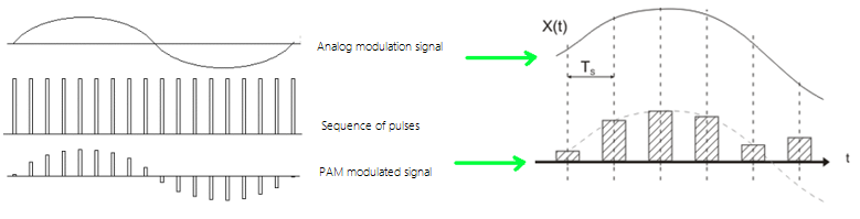
Pulse Amplitude Modulation is a form of modulation where the information message is coded in the amplitude of the carrier pulses.
Therefore, the signal that samples is, generally, a sequence of pulses which amplitudes are proportional to the instantaneous values of the information signal:
Figure 1. PAM modulation process
This type of sampling is called “natural sampling” because the ideal sampling would be made by taking pulses with a duration infinitely small from the modulation signal: this is not feasible in practical terms.
Generally, the natural sampling uses rectangular pulses of very small duration (but finite) for each sample, represented by a sampling pulse.
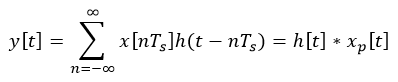
One way to obtain a PAM signal is by sampling the modulation signal, x[n], and convolving with the resultant signal from the sampling,xp[t] , with a rectangular pulse, h[t]:
If T is the period of the modulation signal, and Ts the sampling period, the Nyquist condition will be met if: T=Ts/2. Also, we know that the bigger T is, the smaller bandwidth the modulated signal will have.
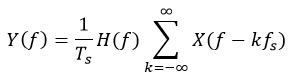
Therefore, the Fourier Transform of a PAM signal is:
Where H(f) is the Fourier Transform of a rectangular pulse:
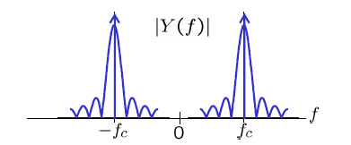
Being τ the pulse width. Therefore, in the frequency domain, the modulated signal is formed by deltas in the fundamental frequency of the carrier and its harmonics, the two deltas corresponding to the modulation signal, a cosine in this case, and deltas in fc ± fm, 2fc ± fm, …
PWM (PULSE WIDTH MODULATION)
In
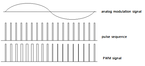
Pulse Width Modulation, the period and amplitude are constant while the modulation signal is going to change the pulses width of the carrier signal, as it is shown in the following picture:
Figure 3. PWM signal generation
The PWM modulation process consists in sampling at regular intervals the information signal and creating a signal with pulses of amplitude constant where the transitions between them happen at regular intervals, while pulses duration depends on the amplitude of the sampled modulation signal.
The PWM technique reduces the noise sensitivity and keeps the same spectrum as a PAM signal for t << T where t and T are the pulse duration and the sequence period respectively.
We can generate a PWM by adding the information signal and a triangular signal:
Figure 4. PWM signal generation (first step)
As we can observe in the image above, the frequency of the information signal is much more lower than the frequency of the triangular signal. The summation or the linear combination of these two signal results in the following signal:
Figure 5. PWM signal generation (second step)
In the previous images, we see an DC component, something that we need to bear in mind when looking at the spectrum.
The next step in the PWM signal generation is to apply a comparator to the last signal and this will results in an output when the voltage is greater than a certain threshold (for instance, 2V) and zero, when is lower. The result is a signal formed by a of variable duration pulses. In the next image, on the left, we have drawn the information signal on top, so you can appreciate the pulse’s width variation according to it: the pulses width increases in the positive cycles of the information signal and vice-versa. On the right side, you can observe the PWM signal.
We can deduce that the spectrum of the PWM signal will have a DC component which belongs to the modulation signal and the spectral components which belong to the triangular signal, with two lateral bands, separated by a bandwidth equal to the modulation frequency:
This structure will be repeated in the multiples of the frequency of the triangular signal.
An additional aspect to bear in mind everytime we sample is the condition that will allow us to reconstruct the signal from its samples: the
Nyquist criteria.
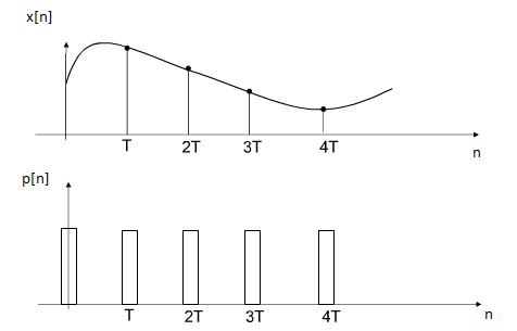
If x
s[n] represent the signal x[n] once is sampled so x
s[n]=x[n]p[n], p[n] is the sampling function that, in this case, we can consider a periodic sequence of pulses (therefore, p[n] can be described using the
Fourier series).
Figure 8. Sampling a PWM signal
The spectrum of the sampled signal, xs[n], is formed by the spectrum of x[n] shifted to the multiples of the sampling frequency. If x[n] is bandwidth-limited, we can get it back by using the Nyquist theorem:
The Nyquist Theorem states that a bandwidth limited signal, x[n], with no frequency components greater than fm Hz, is completely defined by a set of samples taken at a 2xfm Hz rate. Therefore, the time between samples can’t be greater than 1/2 x fm.
If this condition is not met, the signal will show the
Aliasing effect, as we studied in our
previous post, and there will be an overlapping in the signal with its replicas:
Figure 9. Alyasing effect
This implies an incorrect reconstruction of the signal in the time domain. For example:
Figure 10. Aliased signal
We hope you liked this post and be ready for our next Matlab and Simulink tutorial where we will see exercises and code for these two modulations!